Predicting NBA Draft Picks from College Stats

NBA commissioner Adam Silver congratulating point guard Ja Morant, drafted 2nd overall in 2019

Background

The NBA is amongst the most popular and premier sports leagues in the world. Attracting millions of viewers and generating billions in annual revenue, the league truly represents the best of the best in the world of basketball. But the route to the NBA is difficult to say the least. Before getting a chance to play on the biggest stage in basketball, prospective players must prove themselves on smaller stages - whether in the American minor league, internationally, or most often on college courts. Every year, 60 individuals are chosen to join the ranks of the pros in the annual NBA draft. Around 50 or so are drafted directly from college. This selection comes from a pool of over 4,500 Division 1 players across 350 teams. That’s a rate of 1.1%! Part of the spectacle of the draft is that picks are only made public in a televised event at the end of July. Using on-court stats, my goal is to predict which NCAA players will be drafted by NBA teams in a given year and determine which stats best predict draft success.

Dataset

The College Basketball + NBA Advanced Stats dataset on Kaggle contains stats for NCAA Division 1 basketball players from 2009 to 2021. It contains over 60,000 rows representing the seasons of over 25,000 players. Of the 65 columns in the dataset, I chose to make use of 25 and engineered one additional feature: conf_mjr.

Categorical:

conf: Conference

conf_mjr: Conference tier

pos: Position

yr: Year of college

Numeric:

GP: Games played

Min_per: Minutes %

Ortg: Offensive rating

drtg: Defensive rating

usg: Usage rate

eFG: Effective field goal %

TS_per: True shooting %

FT_per: Free throw %

twoP_per: 2-pointer %

TP_per: 3-pointer %

ftr: Free throw rate

TO_per: Turnover %

ORB_per: Offensive rebound %

treb: Average rebounds

dunks: Dunks made

stops: Stops made

bpm: Box plus/minus

mp: Average minutes played

ast: Average assists

stl: Average steals

blk: Average blocks

pts: Average points

Preparation for Model Building

Cleaning and Wrangling

Although the dataset was well organized and not sparse, it required some basic wrangling to reduce the size and deal with missing data and outlier observations. I decided on retaining data from the 2015-2016 season through the 2020-2021 season and removed the columns of all the stats I was not interested in. Given the cardinality of the team feature (362), I decided to drop that column as well. To make things interesting, I also created the feature conf_mjr, which groups the conference a player plays in into either a high, mid, or low competition tier (also called major). My target drafted is a binary variable derived the the pick column signifying a player’s draft status. To avoid data leakage, I dropped the pick column after creating the target and verified that all the stats would be available following the conclusion of a college basketball season. The full wrangle function is included below for reference.

def wrangle(filepath):
  df = pd.read_csv('/content/CollegeBasketballPlayers2009-2021.csv')

  df = df[df['year'] >= 2016].reset_index(drop=True)

  col_drop = ['DRB_per', 'AST_per', 'FTM', 'FTA', 'twoPM', 'ast/tov', 'adrtg', 
              'twoPA', 'TPM', 'TPA', 'blk_per', 'stl_per', 'num', 'ht', 'porpag',
              'adjoe', 'pfr', 'type', 'Rec Rank', 'rimmade', 'midmade',
              'rimmade+rimmiss', 'midmade+midmiss', 'rimmade/(rimmade+rimmiss)', 
              'midmade/(midmade+midmiss)', 'dunksmiss+dunksmade', 
              'dunksmade/(dunksmade+dunksmiss)', 'dporpag', 'obpm', 
              'dbpm', 'gbpm', 'ogbpm', 'dgbpm', 'oreb', 'dreb', 'Unnamed: 65']
  df.drop(columns=col_drop, inplace=True)
  
  df.rename(columns = {'Unnamed: 64': 'pos', 'dunksmade': 'dunks'}, inplace=True)

  # Imputing NaN values
  df['dunks'].fillna(0, inplace=True)

  #Removing outlier observations
  df.drop(index = df[df['Ortg'] > 145.96].index, inplace=True)
  df.drop(index = df[df['eFG'] > 81.3].index, inplace=True)
  df.drop(index = df[df['TS_per'] > 77.8].index, inplace=True)
  df.drop(index = df[df['ORB_per'] > 27.6].index, inplace=True)
  df.drop(index = df[df['ftr'] > 150].index, inplace=True)
  df.drop(index = df[df['drtg'] < 0].index, inplace=True)
  df.drop(index = df[df['bpm'] > 25].index, inplace=True)
  df.drop(index = df[df['mp'] > 40].index, inplace=True)

  #Some feature engineering 
  def set_major(conf):
    high_major = ['B10', 'SEC', 'ACC', 'B12', 'P12', 'BE']
    mid_major = ['Amer', 'A10', 'MWC', 'WCC', 'MVC', 'CUSA', 'MAC']
    if conf in high_major:
      return 'high'
    elif conf in mid_major:
      return 'mid'
    else:
      return 'low'
  df['conf_mjr'] = df['conf'].apply(set_major)

  # Creating the target column
  df['drafted'] = df['pick'].notnull().astype(int)
  df.drop(columns='pick', inplace=True)
  df.sort_values(by='year', ascending=False, inplace=True)
  draft_picks = df[['pid', 'drafted']][df['drafted'] == 1]
  late_draft_ind = df.loc[draft_picks[draft_picks.duplicated()].index].index
  df.loc[late_draft_ind, 'drafted'] = 0

  # Dropping high-cardinality team column
  df.drop(columns=['team'], inplace=True)

  # Dropping rows with any null value
  df.dropna(axis=0, how='any', inplace=True)
  df.drop(index = df[df['yr'] == 'None'].index, axis =0, inplace=True)

  df.drop(columns = ['pid'], inplace=True)
  df.set_index('player_name', inplace=True)
  
  return df

Splitting the Data

I decided to do a time-based split and separate the data into the following 3 subsets:

Training set containing stats from 4 seasons (2016-2019)
Validation set containing stats from the 2020 season
Test set containing stats from the 2021 season

cutoff = 2020
df_train = df[df['year'] < cutoff]
df_val = df[df['year'] == cutoff]
df_test = df[df['year'] > cutoff]

X_train = df_train.drop(columns = [target, 'year'])
y_train = df_train[target]

X_val = df_val.drop(columns = [target, 'year'])
y_val = df_val[target]

X_test = df_test.drop(columns = [target, 'year'])
y_test = df_test[target]

Baseline

To establish a baseline, I calculated the relative frequency of the majority class for both the training and validation set.

baseline_train_acc = y_train.value_counts(normalize=True).max()*100
baseline_val_acc = y_val.value_counts(normalize=True).max()*100

Unsurprsingly, predicting that zero players get drafted nets an accuracy score of 98.91% for the training set and 98.92% for the validation set. Even though accuracy will not be the primary metric of evaluation, it will be interesting to see how different model perform in this respect. Since the classes are so imbalanced and my focus is on classifications of the positive class, precision/recall and particularly the F1 metric will be crucial.

Classification Models

Logistic Regression

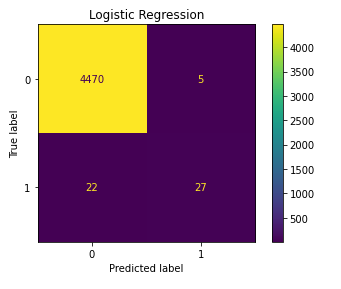
The first model I ran was a linear model - logistic regression with default parameters. Right off the bat, the bare-bone model had a validation accuracy of 99.40%, a whopping 0.48% above baseline. And with a precision of 0.84 and recall of 0.55 combining to give an F1 score of 0.67, these metrics were the ones to beat. As shown in the confusion matrix below, the model correctly predicted 27 out of the 49 college draft picks in 2020 and only misclassified 5 players into the positive class. For such a simple model, that’s not too bad!

Tree-based Models

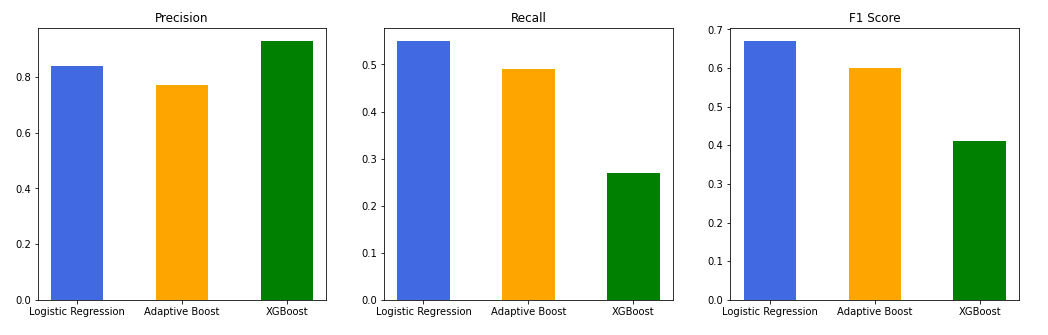
I trained 5 tree-based classification models, also with default parameters, to see how they would handle the severe class imbalance: a basic decision tree, a bagging model (Random Forest), and 3 boosting models (Adaptive Boost, Gradient Boost, and Extreme Gradient Boost). The random forest model fared the worst with an meager F1 score of 0.19 - a combination of perfect precision and terrible recall scores. Despite having a validation accuracy below baseline, the decision tree did an overall better job (F1 of 0.40) and “took more chances” at predicting a positive draft status. The AdaBoostClassifier performed the best out of the lot with an F1 score of 0.60 and accuracy of 99.29%, well above baseline. The GradientBoostingClassifier and XGBoostClassifier perfomed similarly with respective F1 scores of 0.43 and 0.41.

Initial Model Comparison

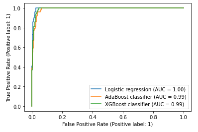
Out of the 6 models, I decided to compare the logistic regression, AdaBoost, and XGboost classifiers as candidates for the final model. One method of comparing binary classifiers is to plot their respective ROC (receiver operating characteristic) curves. Even though the curves shown below are extremely tight given the uneven distribution of my target, any marginal differences would be informative. The logistic regression model had the highest area under its curve (0.996) which was unsurprising given that it had the highest accuracy and F1 score. The XGBoost AUC came out to 0.993 while the AdaBoost classifier scored the lowest at 0.990.

Hyperparameter Tuning and Final Model Comparison

Utilizing a 5-fold cross validation, I used grid-search to find the optimal set of hyperparameters for the 3 models in the specified search spaces. The metric used to score the different iterations is the F1 score.

model_log = make_pipeline(OneHotEncoder(use_cat_names = True),
                          StandardScaler(),
                          LogisticRegression(n_jobs=-1, random_state = 42)
                          )
param_grid = {'logisticregression__max_iter': [100, 200, 300],
              'logisticregression__solver': ['newton-cg', 'lbfgs', 'liblinear'],
              'logisticregression__penalty': ['none', 'l1', 'l2', 'elasticnet'],
              'logisticregression__C': [10, 1.0, 0.1]
              }
model_log_s = GridSearchCV(model_log,
                          param_grid=param_grid,
                          n_jobs=-1,
                          cv=5,
                          scoring='f1',
                          verbose=1
                          )
model_log_s.fit(X_train, y_train)

model_ada = make_pipeline(OrdinalEncoder(),
                          AdaBoostClassifier(
                            base_estimator=DecisionTreeClassifier(),
                            random_state=42)
                          )
param_grid = {'adaboostclassifier__base_estimator__max_depth': [1,2],
              'adaboostclassifier__learning_rate': [0.1, 0.5, 1],
              'adaboostclassifier__n_estimators': [50,100,150]
              }
model_ada_s = GridSearchCV(model_ada,
                           param_grid=param_grid,
                           n_jobs=-1,
                           cv=5,
                           scoring='f1',
                           verbose=1,
                            )
model_ada_s.fit(X_train, y_train)

model_xgb = make_pipeline(OrdinalEncoder(),
                          XGBClassifier(n_jobs=-1, random_state = 42)
                          )
param_grid = {'xgbclassifier__scale_pos_weight': [1, 10, 50, 99],
              'xgbclassifier__learning_rate': [0.01, 0.1, 0.3],
              'xgbclassifier__max_depth': [3,6,9],
              'xgbclassifier__n_estimators': [50,100,150]
              }
model_xgb_s = GridSearchCV(model_xgb,
                           param_grid=param_grid,
                           n_jobs=-1,
                           cv=5,
                           scoring='f1',
                           verbose=1
                           )
model_xgb_s.fit(X_train, y_train)

Pre-tuning:

Post-tuning:

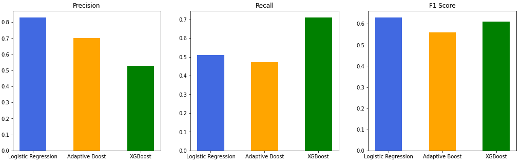
Tuned Model	Accuracy	ROC AUC	Precision	Recall	F1 Score
Logistic Regression	99.358974	0.996393	0.83	0.51	0.63
Adaptive Boost	99.204244	0.981694	0.70	0.47	0.56
XGBoost	99.005305	0.993492	0.53	0.71	0.61

From the above plots, we can see that XGBoost classifier benefitted the most from tuning. Both precision and recall increased substantially, giving an F1 score on pace with the logsitic regression model!

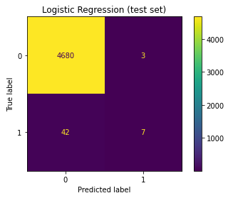
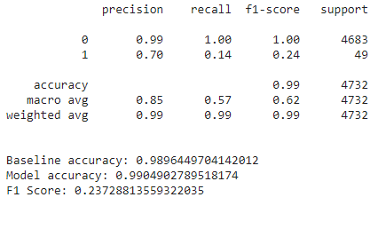
Final Prediction

For my final model, I decided to go with the logistic regression. Below are the prediction results of the 2021 draft in a confusion matrix format as well as the classification report. Surprisingly, the linear model did much worse on the test set than on the validation set!

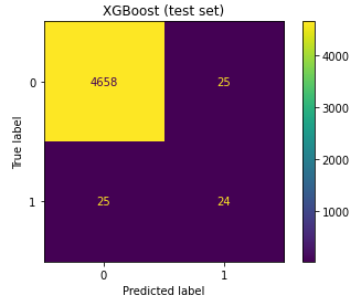
Seeing that the logistic regression model did not perfrom all that well on the test set, I decided to cheat and run the test set on the updated XGBoost as well. Here are the results:

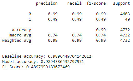Looks like I chose the wrong model!

Important Features

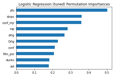
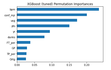
Concluding Thoughts

Over the past decade, the NBA and college basketball programs have increasingly embraced the power of data analytics. In fact as of 2020, almost every professional team has a department in their front office dedicated specifically to analyzing data. With this project, my goal was to explore this territory at the intersection of sports and data science by building a basic model to predict draft outcomes of college players using on-court stats. However, I’m sure stats are far from the only factors that that go into draft decisions. One main factor that is not accounted for is the kind of player a team is looking to add to its roster in any given year. Another may be personality. Though ultimately, skill and ability on the court are king. And stats are the best way to capture that.

Looking forward, some potential improvements to building a better model could be:

finding the right combination of stats to train on
handling 0s and 1s for percentage features better or dropping those observations altogether
adding a feature to distinguish draft-eligible players
adding a feature to distinguish players who have actually declared for the draft
adding or calculating a composite score feature

A methodology of undersampling or oversampling could also used on the dataset to mitigate the effects of the extreme class imbalance on the modeling process. It would also be interesting to build a regression model to predict not only which players will be drafted but the order in which they are chosen!